The idea, in three panels
This is the whole method, seen at once. A campaign is drawn as a river: 1592.60 to 1594.60 nm of TOI-2120, one row per exposure, 316 of them, stacked in order of barycentric velocity and drawn in the star's rest frame. That frame is the trick of the picture: vertical structure belongs to the star; anything slanted does not. The eye separates them before any arithmetic does.
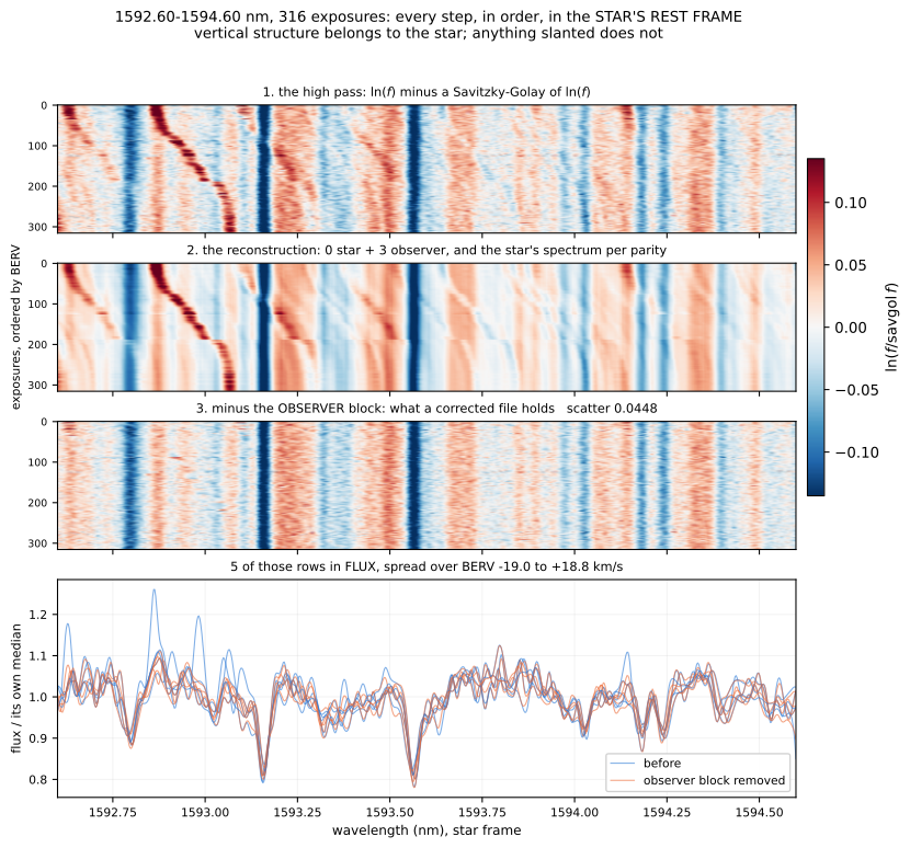
- 1. What arrives. The log of the delivered flux, less a Savitzky-Golay of it, which takes the continuum off and leaves the lines. The star's lines are the vertical ones. The bright diagonal crossing them is OH airglow, sky emission that sits at a fixed place on the detector and therefore sweeps across the star as the Earth's velocity changes over the year.
- 2. What the model says is there. One basis fitted in the star's frame and one in the observer's, solved together for every exposure at once. The reconstruction has the star's vertical lines and the sky's diagonal ones, each where it belongs, because the model was told which of the two travels.
- 3. What a corrected file holds. Panel 1 with the observer block divided out of it. The diagonal is gone and the vertical lines are untouched: the star was never in the block that was removed. That panel is not an illustration of the correction, it IS the correction, sample for sample, and a test keeps the two together.
The model behind it
That is what the picture above is: over a year of observing, the barycentric velocity sweeps by tens of kilometres per second, which is enough to separate the star from the atmosphere, but only if the model is told which of the two travels. In one line, Each exposure is the log of its flux less a Savitzky-Golay of it (a 100 km/s high pass, 201 samples of 0.5 km/s; runs made before 2026-09-11 used 151 of them, 75 km/s), on one log-uniform grid in the observer's frame, as two rows, its even orders and its odd ones:
y_n = S_n P a_n + v_n d(S_n P a_n)/dv + Q b_n + m_pS_ncarries the star basisPinto exposurenby its barycentric velocity. On a log grid a Doppler shift is a translation of atanh(v/c)/(dv/c) samples, relativistic, andS_nis an exact Lanczos operator for it rather than an interpolation that would smear what it touched.P a_nis the star;Q b_nis what stands still on the detector: telluric absorption, OH emission, the instrument.v_nis one velocity per exposure, times the derivative of the star as reconstructed. Without it the observer block learns the star's own motion and the correction divides it out of the flux. With it the motion is fitted, and stays in.m_pis one offset per order parity, in the observer's frame. Consecutive orders overlap, and at a given wavelength one parity samples near an order's centre and the other near its edge, where the resolution differs. It is taken out before the fit and put back into the correction.
The coefficients of both blocks are solved together for each exposure, under weights taken from the noise you can measure rather than the noise a photon model claims. The two disagree by a factor of fifty at the red end of a SPIRou spectrum: past about 2200 nm the thermal background dominates, the pipeline subtracts its mean and not its variance, and a photon model computed from what is left reports the noisiest part of the detector as the quietest.
What a corrected file holds
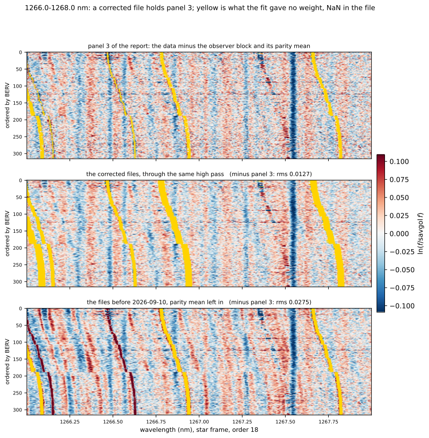
Panel 3, sample for sample. A corrected file is the delivered flux
times exp(−(Q b_n + m_p)) on its own pixels, and
NaN wherever the fit gave a sample no weight, so LBL is never handed
data the model never saw. The star block and the velocity term stay
in: they are what LBL is about to measure. Everything else in the
t.fits, wavelength solution and blaze included, is copied through.
Install it
One conda environment, described by the repository itself, and five lines. It holds both codes, this one and LBL, because having to deactivate one to run the other is how a t.fits gets measured by the wrong version of something.
git clone https://github.com/eartigau/pca2d_preclean.git
cd pca2d_preclean
conda env create -f environment.yml
conda activate pca2d-preclean
./check.sh
One alias, written once, so that a new terminal is one word from being ready:
echo "alias pca2d='source $PWD/pca2d.sh'" >> ~/.zshrc
pca2d then leaves whatever conda environments are active,
however many deep, enters this one, and prints what there is to run.
Leaving rather than activating on top is the point: the environments
that matter here hold versions of LBL, and the wrong one on the path is
how a t.fits gets measured by the wrong version of something.
./check.sh is the check that it worked: 489 tests, about
thirteen seconds, and not one spectrum or network call among them. Then put the spectra of
a target in data/<object>/ under the input root,
which is never written to, and either
pca2d-preclean --object TOI-2120     # the whole thing, t.fits to velocities
pca2d-gui                            # the same, in a window
The environment pins rather than floors its versions, because LBL pins
its own exactly: numpy==2.3.3, astropy==7.2.0,
scipy==1.17.0 and the rest, python 3.12.
environment.yml repeats those pins so that conda installs
them and pip finds them already satisfied. The repository itself is
private for the moment: the clone needs access, which
is a message away. And if
conda env create ends in Pip failed, the
reason is almost always the one at the foot of this
page, which has nothing to do with this package.
The window
pca2d-gui
For anyone who should not have to read a command line before their
first run. It does nothing the command line cannot: every setting is
one key of config.yaml or one flag of
pca2d-preclean, and the command it is about to run
is written out in full, so it can be read before anything
happens and copied into a terminal afterwards. It runs that command as
a subprocess, shows its output as it comes, and can stop it. It came
with the package you just installed, so that one word is the whole of
starting it.
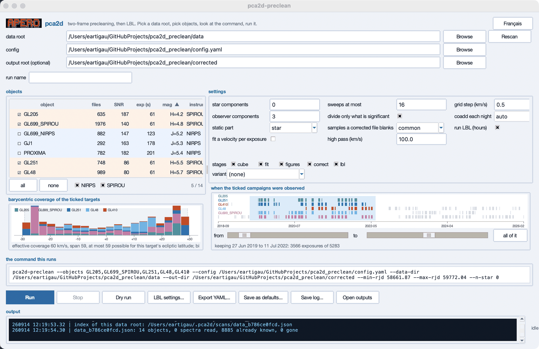
--min-rjd and --max-rjd: that
is how a campaign is cut into seasons.
Three pages
Everything at once was a wall. The window is four pages, and each has room to be read: targets, what is being reduced; settings, how; LBL, what the step that produces velocities is asked; and analysis, the command, the buttons that start and end it, and everything it says. The banner and the language button stay above them.
Two roots, and one file written in the first
A data root, shown in full, since data means different
folders from different working directories and a campaign usually lives
behind a link onto a shared disk. The only thing ever written there is
one pca2d_index.csv per campaign folder, the log of what
has been read of that campaign; the spectra are never touched, and a
folder that refuses the file stays exactly as it was. An output root, proposed as
corrected beside the data root when the field is left
empty: the corrected spectra are a copy of the campaign, tens of
gigabytes, and belong on the disk the campaign is already on. A
reduction name, which names the folder the run writes
into. It is proposed rather than left empty, as the targets followed by
six characters of a hash of everything that makes this reduction a
different result: the component counts, the velocity term, the sweeps,
the shrinkage, the high pass, the grid step, the coadding and the date
window. The same parameters give the same six, one number different
gives another six, and the window says when a reduction of that name
already exists rather than letting it be found out afterwards.
A window opened for the first time has both roots empty
and its configuration set to the config.yaml that came with
the installation, found beside the package rather than resolved against
whatever folder the window was started from. Where the spectra are and
where their copies go are choices about somebody's disks, and a field
that opens with a plausible path in it invites a run against a folder
nobody picked. The status line says pick a data root for as
long as there is none, the log says what such a folder holds, and the
command box says tick a target rather than showing a command
with no --object in it.
The targets, and what is known about them
The list is one row per campaign folder: the number of spectra, the
median signal-to-noise, the median exposure time, the magnitude with
the band it is in, and the instrument. Rows are grouped and tinted by
instrument, a column heading sorts by that column and again to reverse
it, the object heading a third time for the default order, and what is
not known sorts last, never first. A campaign still being read carries a disc
beside its tick box, filling clockwise as its files come in and gone
once they all are, so a finished list is not a column of symbols. A tick box per row, with
all, none, a double-click or the space bar,
and a count of what is ticked against what is listed. The boxes under
the list show or hide one instrument's targets.
Those numbers come from the headers, so the first visit to a data root
reads one header per spectrum: the per-order extraction signal-to-noise
APERO wrote (EXTSNxxx), the exposure time, the barycentric
velocity, the coordinates, the magnitude under whichever keyword that
instrument writes, and INSTRUME, which is read from the
FILE and never from a configuration. The answers go into one index per
root under ~/.pca2d/scans/, named after the root with a
digest of its full path, so two roots whose last folder is called
science cannot share one index.
The same answers are written beside the data, as a
pca2d_index.csv inside each campaign's own folder: one line
per spectrum with the keywords read from it, appended every ten files
and rewritten when that campaign is finished. Inside the folder rather
than at the top of the root because campaigns are copied one at a time,
and a log that stays behind is a campaign read again at the other end.
That is what a second window reads, on this machine or another one
mounting the same disk, so a campaign is read once by whoever gets there
first. The header row is the schema, so a log
written by a version with other columns is ignored rather than half
believed, and every line is still checked against its file's size and
modification time before it is used.
Every later visit draws the list at once from that index, then checks the root: a file is taken as it was if its size and modification time are unchanged, and only what was added or replaced is read, which is what Rescan does after copying new spectra in. The window also does it for itself, every ten seconds: one folder listing per campaign, nothing opened, so a campaign copied in while it sits open turns up on its own rather than the next time somebody thinks to press Rescan. The names and the file counts appear before a single header is read, since they cost one folder listing. A campaign's first numbers arrive from ten spectra spread across it rather than the first ten, and carry a tilde until the rest are in: file names sort by date, and the first ten of a campaign are one night's weather. On GJ 1 they give 134 against the campaign's 163. A field added to the index re-reads the files that lack it and only those, a file that cannot be read is recorded as unreadable rather than retried at every visit, and deleting an index costs the few seconds of one scan and nothing else.
One target, or several against one observer basis
Tick one box for a solo run. Tick several and they are fitted together against a single observer basis, each star keeping its own spectrum per order parity. The atmosphere and the instrument belong to the night rather than to the target, and no basis can follow one star when several, with different barycentric coverage and systemic velocities, constrain it. They must come from one instrument: two ticked instruments refuse to run, because a run is one domain, one grid and one set of extensions, all read from the instrument. The window reports how many nights the ticked campaigns share, as information and not as a requirement: the observer components are a parasite that is always present, what a fit measures is their pattern, and nights no other star of the group saw widen the range of conditions that pattern is measured over.
What the sky allows, before anything is run
Under the list, the barycentric coverage of whatever is ticked, as a histogram in bins of 3 km/s stacked by star, with three numbers: what the campaign covers, its span, and what the target's ecliptic latitude ALLOWS. That last one is fixed by the solar system, |BERV| ≤ 29.78 cos(β), and it decides whether the method can work on that target at all: TOI-1452, at +80.5 degrees, can never span more than 9.8 km/s. A coverage short of the span means gaps, which more nights fill; a span short of what is possible means a young campaign; a small possible means the wrong target. It is the most useful thing on the window to look at before starting a twenty-minute run, because the correction is worth about a factor of two where the span is wide and costs about as much where it is not.
Under it, the signal-to-noise against that same velocity, one dot per spectrum in its star's colour. The histogram says which velocities a campaign covers; this says what it covers them with, and the fit weighs a spectrum by 1/sigma²: a range whose far end is covered by a campaign's worst nights is not the range the fit really sees.
Beside it, when the ticked campaigns were observed: one mark per exposure in its star's colour against a calendar axis, and two sliders that keep a date window, with a line underneath saying what is kept and how many exposures of how many that is. What falls outside is neither fitted nor corrected, which is how a campaign is cut into seasons and how the two ends of a baseline are compared. all of it puts the window back to the whole campaign, which is the nominal path.
The settings that change a result, and only those
How many components in each frame, whether a velocity is fitted per exposure, how many sweeps at most, whether only the significant part of the correction is divided out, the high pass, the grid step and nightly coadding. Resting the pointer on one writes what it means at the bottom of the window, and after a moment in a box: the explanations are the ones in the documentation, not a restatement of the label. Nothing cosmetic is on this panel, on purpose, and neither is anything settled: the star is one cubic B-spline, the static part is one star spectrum per order parity, and a sample lost by one exposure comes back as NaN in all of them so that the campaign carries one set of lines. All three are fixed in the code, so the window does not ask. The older modes are still read from a config or a variant file, for redoing the runs that were measured on them. Whether LBL is run, which is hours of work, is in the LBL window: the stages already say whether the lbl step happens at all.
The stages are drawn as the chain they are,
cube → fit → correct → lbl,
because that is the order they happen in and the order they depend on
each other in: unticking one unticks everything after it, and ticking
lbl ticks the correct it measures. Ticking does
not pull the chain the other way, so a fit can still be reused and only
the correction redone. figures sits apart on the same line
with no arrow to it: it draws what the fit left, and nothing waits for a
drawing. There is no variant picker: the parameters
converged, and a second set of settings offered beside the settings is a
window that contradicting itself. A variant is still a file and still
runs, from the command line.
The LBL page holds the lbl: block: what
is measured (the delivered spectra, the corrected ones, or both), what
the corrected object is called next to the delivered one, which template
it is measured against, where LBL's tree is, which of its steps run,
whether LBL is actually run, and whether the spectra get there as
symlinks or as copies. That is the equivalent of the wrapper script, and
it is the step that produces velocities.
What it writes, and what it remembers
- Dry run resolves everything, says what it would do, and touches nothing.
- Export YAML saves the settings that differ from the configuration as a variant file, which is how one run is made reproducible. A variant that repeats the nominal says nothing, and the window refuses to write one.
- Save as defaults writes those same settings into
config.yaml. It edits the lines it has to and nothing else, so the comments that say which measurement chose each value survive, where ayaml.safe_dumpof the parsed document would have deleted all of them. It asks first, and shows exactly which keys it is about to change. - Save log writes what the window has shown. The run
prints there as it goes, in the colours it uses in a terminal, green
for progress, blue for a number, orange for something skipped, red for
what stops a run, and the window's own lines take the same form,
YYMMDD HH:MM:SS.SS | message. - Open outputs opens the folder the run is writing into.
- Quit, at the other end of the bar from Run, closes the window. The settings are written at every change, so nothing is lost by leaving; a run is a subprocess of the window and is stopped by leaving, so it asks first, and so does the window's own close box.
English or French, one button, everything included: the
labels, the explanations and the log lines. The window holds no state of
its own beyond the last settings and what was ticked, in
~/.pca2d_gui.json, and the per-root index under
~/.pca2d/. It does not resolve the configuration itself,
never touches the data, and every choice it offers exists on the command
line, which is what the box at the bottom is there to prove.
LBL, built in
The corrected spectra exist to be measured, and the only honest way to
know whether the correction helped is to measure both. The
lbl stage puts two objects side by side in
one LBL tree: TOI-2120, symlinked to the spectra as
delivered and measured against the template LBL builds from them, and
TOI-2120_PCA2D_1-3v, symlinked to what the run corrected.
The name carries the run's tag, because LBL takes a whole science
folder and two corrections in one would be measured as a single series
without a word.
The corrected object's template is the fit's star. The first star component at its mean amplitude is a high-passed template of the star, fitted to every exposure at once with the atmosphere already described by the other block. Each order parity gets its own, the star block plus that parity's weighted mean of what the fit left, since LBL measures an order against the template of its parity. The stage writes it in LBL's template format, by LBL's own writer, and puts it where LBL looks for that object's template, so LBL's template step finds it and has nothing to do. A template LBL built itself is never replaced. Through the 75 km/s high pass of the day it was measured, it agrees with LBL's own template for the same spectra at a correlation of 0.93 and a slope of 0.94, and 0.99 and 0.99 in H.
The star components past the first are variability
indicators, and LBL already knows what to do with those: it
projects every line's residual on RESPROJ tables, its DTEMP temperature
gradients. With two or more star components the stage writes the
others as the same tables, STRPCA2 to
STRPCAn, measured on the star itself rather than taken
from a model, and the rdb gets each exposure's amplitude along them and
its error. LBL reads those tables in the star's rest frame, which its
mask step measures, so the corrected object's mask is made first, then
the tables, then the velocities.
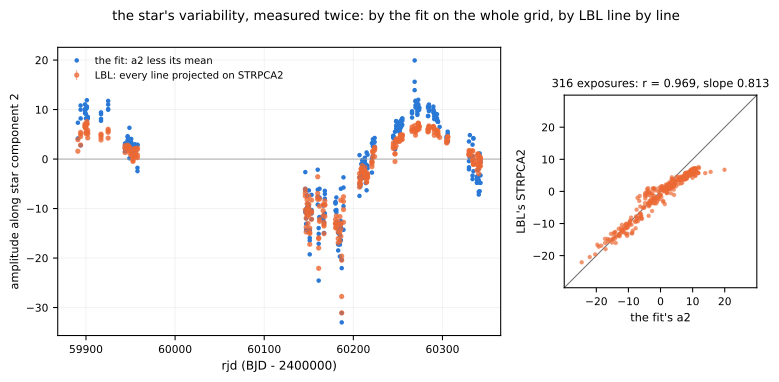
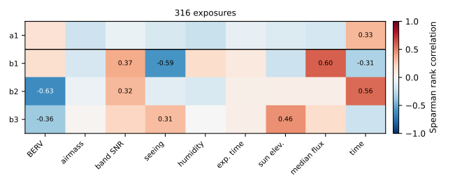
That same fit is also the warning that goes with it. Its a2 follows the barycentric velocity (−0.55), the seeing (−0.58) and the sun's elevation (−0.49): a star component modelling the sky. Its velocity term absorbed shifts of 232 m/s rms that follow the barycentric velocity, the correction left that in the flux, and LBL's velocities on those spectra scatter by 67 m/s, against 27 with one star component. A second star component is a variability indicator once the correlation table says it belongs to the star.
What the stage leaves is meant to be read and rerun by hand:
lbl_config.yaml in LBL's own keys, and
run_lbl.py, an ordinary LBL wrap script with one runparams
dict per object. lbl.run: true or --run-lbl
has the stage run it.
What the coefficients do in time
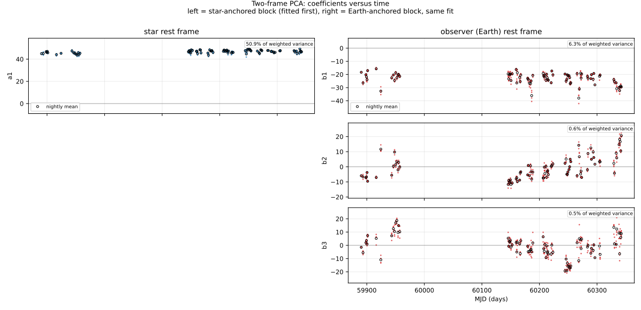
One component in the star's rest frame, three in the observer's, one point per exposure over 452 days.
And what they follow
A component carries no label. That one varies is a result; what it varies with says what it is describing. Every run writes this matrix without being asked, because it is the diagnostic that catches a "stellar" component quietly modelling the sky.
Running it
Spectra go in data/<object>/ under the input root and
everything a run writes goes under the output root, so the archive it
reads is never the folder it writes to. Then:
pca2d-preclean --object TOI-2120
That is the whole interface. The instrument is read from the
INSTRUME keyword of the files, never chosen on a command
line, because reading the wrong extension raises no error: it returns
different photons. Five stages, cube, fit,
figures, correct and lbl, each
announcing how long it took. On 316 SPIRou exposures the fit, the
report and the correction take twenty to thirty minutes, and LBL about
half an hour per object.
output.fits_directory keeps a run's products on another
disk: the run folder, and every LBL folder but the one made of
symlinks, become links to it before anything is written, and a run
stops rather than write locally when that disk is not there.
Adding a spectrograph
A block in config.yaml, not a line of code:
instruments:
  YOURS:
    extensions:
      flux: FluxAB
      wave: WaveAB
      blaze: BlazeAB
      recon: Recon
      sky: OHLine
    domain:
      wave_min: 955.0
      wave_max: 2500.0
      wave0: 955.0
    lbl:
      instrument: SPIROU
      data_source: CADC
The wavelength solution comes from the extension, never from header
polynomials, and the blaze from the blaze extension of the same file.
LBL's name for the spectrograph goes with it: LBL calls NIRPS
NIRPS_HA or NIRPS_HE by the mode it was
observed in, and the wrong one raises no error.
What comes out
- outputs/<object>/<tag>/<object>_<tag>.pdf: one multipage document, the resolved parameters as selectable text first, then every figure, with bookmarks.
- fit.npz, twoframe_components.fits, the coefficients as CSV, and resolved_config.yaml: exactly what ran, next to what it produced.
- corrected/: the corrected spectra, one per input file, each saying in its header what was divided out of it and carrying every amplitude the fit has.
- star_template.fits, lbl_config.yaml and run_lbl.py: LBL set up on both sets of spectra, the corrected ones against the fit's own star.
The tag is the number of star and observer components, and
v when the velocity term was fitted: 1-3v
above.
What it is worth, measured
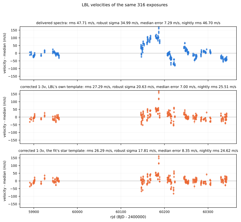
Everything above is a method; this is what it does to the numbers that matter. TOI-2120, 316 SPIRou exposures over 452 days, corrected with one star and three observer components, then measured by LBL on the same exposures before and after:
| spectra | template | rms | robust sigma | nightly rms | median error |
|---|---|---|---|---|---|
| as delivered | LBL's own | 47.7 m/s | 35.0 m/s | 46.7 m/s | 7.29 m/s |
| corrected, 1-3v | LBL's own | 27.3 m/s | 20.6 m/s | 25.5 m/s | 7.00 m/s |
| corrected, 1-3v | the fit's star | 26.3 m/s | 17.8 m/s | 24.6 m/s | 8.35 m/s |
When the install fails
One failure is common enough to name, because nothing in its message
points at its cause. conda env create ends with
CondaEnvException: Pip failed, and above it:
× git version did not run successfully.
  xcrun: error: unable to load libxcrun
  (/Library/Developer/CommandLineTools/usr/lib/libxcrun.dylib:
   fat file, but missing compatible architecture (have 'arm64,arm64e', need 'x86_64'))
ERROR: Failed to build 'git+https://github.com/njcuk9999/lbl@main'
It is not LBL, and it is not pip. The environment is x86_64,
running under Rosetta on an Apple Silicon Mac.
environment.yml asks pip for LBL from git, pip runs
git, Apple's /usr/bin/git is a stub that calls
xcrun, and xcrun loads
libxcrun.dylib, which on recent Command Line Tools ships
arm64 slices only. An x86_64 process cannot load an arm64 library, so
git version fails and conda reports the only thing it saw,
which is that pip failed. Nothing here is specific to this package: any
environment that pip-installs from a git URL hits it.
Three lines that say whether that is what happened
uname -m                                   # the shell:      arm64 on Apple Silicon
conda activate <env>
python -c "import platform; print(platform.machine())"   # the environment
conda config --show subdir                 # osx-arm64, or osx-64 under Rosetta
Three answers that agree on arm64 and
osx-arm64 mean this is not your problem. Any
x86_64 or osx-64 among them is the cause.
The fix worth doing
Rebuild the environment natively. It is not only the way out of this error: LBL is hours of arithmetic, and hours of arithmetic under emulation are longer hours.
CONDA_SUBDIR=osx-arm64 conda env create -f environment.yml -n pca2d-preclean
conda activate pca2d-preclean
conda config --env --set subdir osx-arm64   # so later installs stay native
And check the terminal itself, since an environment inherits the
architecture of the shell that made it: Finder, Applications, Terminal,
Get Info, and Open using Rosetta must be unticked. If
uname -m says x86_64, look there first.
Two ways round it, if the environment has to stay x86_64
- Give the environment its own git, of its own architecture, so pip
stops reaching for Apple's stub:
conda install -n <env> -c conda-forge git. - Or take git out of the install: clone LBL by hand and point pip at
the folder,
git clone https://github.com/njcuk9999/lblthenpip install -e ./lbl.
Access
The repository is private for the moment. If you would like access, or would like to try it on a dataset of your own, contact Étienne Artigau (Université de Montréal). This page stays public so the method and its figures can be pointed at.